Around 3 weeks ago, I attended the Machine Learning Research School (MLRS) 2019 in Bangkok, Thailand. The event basically includes lectures of the topics relevant to Artificial Intelligence (AI) and Machine Learning (ML). But one particular topic that I was looking for the most was Causal Inference taught by Elias Bareinboim. It’s one aspect of data science that is crucial but not taught widely enough in my opinion. I only became aware of this area only recently as well. So, this blog is my attempt to raise awareness on this topic and, perhaps, help better the practice of data science in general.
What is Causal Inference (CI)?
You’ve probably heard the catchphrase “correlation is not causation” before. But what does it mean to infer causation? The process of inferring causal relationships is called causal inference. This process is needed when we want to know whether a certain event/action causes another and doesn’t just correlate with or predict it. Still, we usually use statistical techniques to determine the causal effect. But statistics alone cannot inform us about causality (or anything really).
Causal Diagrams with the third variable
Let’s take a look at an example used in Elias’s lecture at MLRS (with a slight modification). Let’s say we obtain a dataset containing data of people with a serious illness. The data indicates whether patients taking a drug (treatment) and whether they survive after taking the drug (outcome). We go ahead and explore the data and create a table showing statistics of recovery rate as in figure 1.
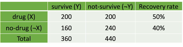
figure 1. table showing recovery rate of treatment and control groups
From figure 1, it seems that patients who take the drug have better chance of surviving. But when we later take into account the variable age of the patients (here we split into a group of adults and children), it results in the tables with different story to tell like in figure 2.
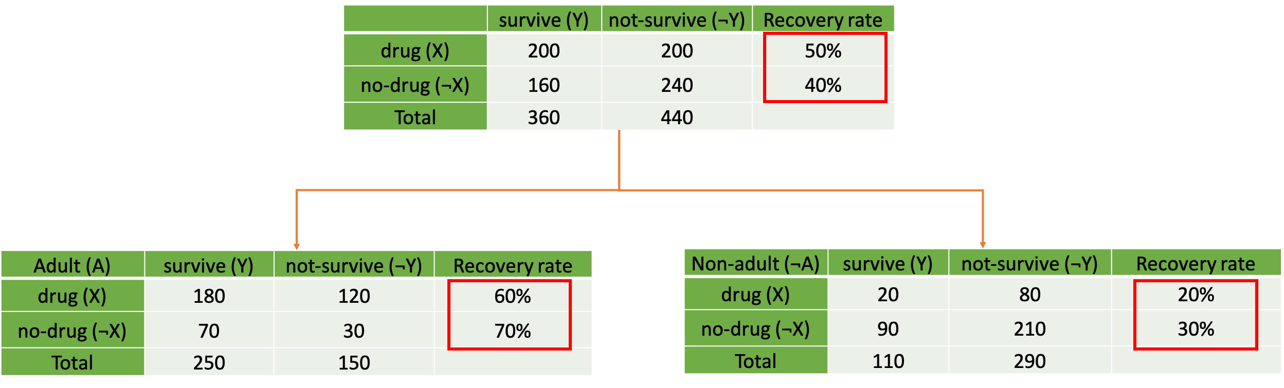
figure 2. table showing recovery rate of treatment and control groups separated by age (Adult vs Non-adult)
From what we can notice from the tables in figure 2, it seems that the patients are more likely to survive by not taking the drug for both adults and children now. This is a phenomenon called Simpson’s paradox. This phenomenon happens when some subgroup variables are neglected in the analysis resulting in a disappearance or reversal of patterns in the data. This phenomenon can be generally attributed to “confounder” variables. So, how do we prevent this from happening in the first place? We have to remember that statistics is just a tool. Analysis results can’t tell us anything without our assumptions or contexts. In a causal inference framework, Structural Causal Models (SCM), we express our assumptions using a causal graph, which is basically a Directed Acyclic Graph (DAG). Considering our example, there are 3 main potential causal graphs that would give us results as in figure 2. These three causal graphs are illustrated below in figure 3. Each of them reflects different assumptions of how the world works, or how taking the drug, age, and survival rate relate to one another in this scenario.
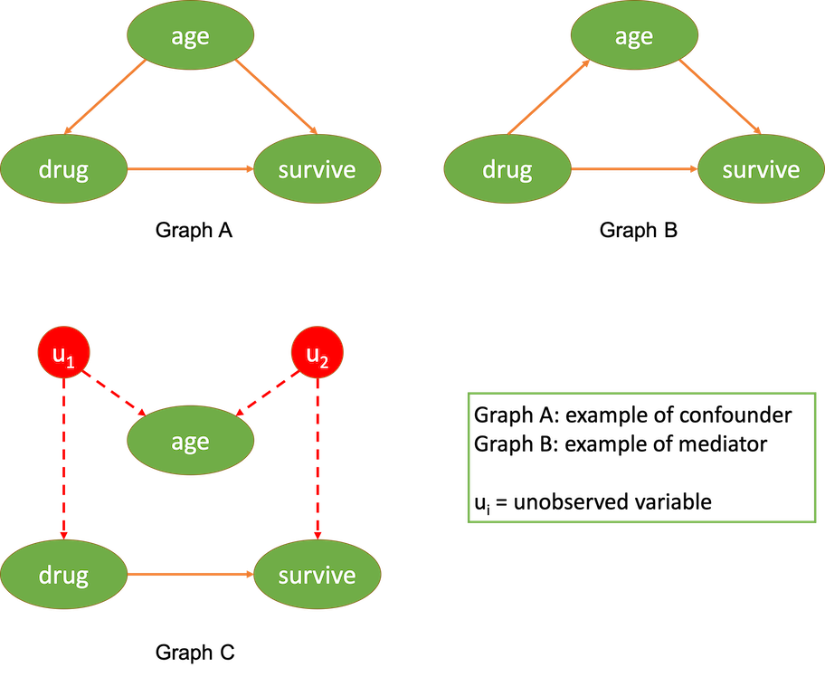
figure 3. example of causal graphs
According to figure 3, our first potential causal graph (graph A) indicates that the age variable is a confounder variable between the treatment and outcome variables. This means that the age variable partially determines who do (or do not) take the drug while it also influences the survival rate (adults and children have different base survival rate). Whereas, the second causal graph (graph B) reflects that the age variable partially mediates the effect of the drug on survival rate. But we can use our intuition to filter out this possibility because the drug (usually) shouldn’t be able to make adults biologically equivalent to children and vice versa. Lastly, graph C indicates that the relationships between drug, age, and survival rate are confounded by unobserved variables. Learning from this example, you might start thinking that we should throw in as many variables into the analysis as possible. But there’s another type of variables in the causal framework that’s called a collider. A collider variable in a causal graph will look like in figure 4 below.
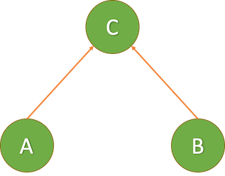
figure 4. causal diagram of a collider (variable C)
A collider variable is a variable that you must not incorporate into your analysis because it will produce a relationship between your variables of interest when there is none. From figure 4, variable C is a collider variable and it will establish a link between variable A and variable B if you include it in your analysis even though there’s no direct link between A and B. Another article here will give you a clearer example of colliders (Rohrer, 2018).
Causal hierarchy and identification
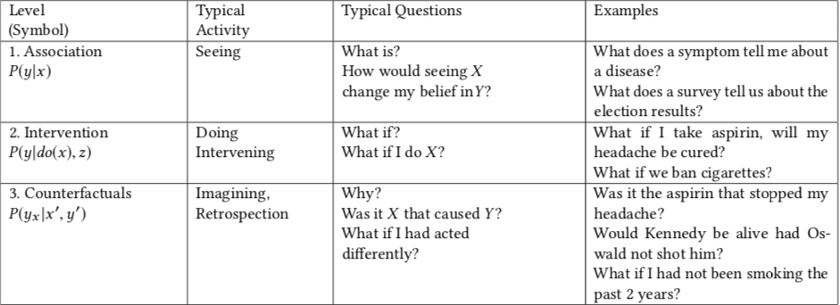
figure 5 Judea’s causal hierarchy showing different level of causal questions ([source](https://dl.acm.org/doi/10.1145/3241036))
According to Judea’s causal hierarchy, there are 3 levels of causal questions we can ask, including association, intervention, and counterfactual. This model is described as a hierarchy because if you have access to information at the higher levels, it’s implied that you can answer the queries at the lower levels as well. The lowest level of this hierarchy is association that includes correlational analyses and most predictive models (Pearl, 2019).
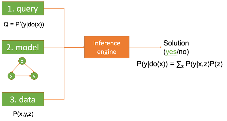
figure 6. causal inference engine in Structural Causal Model
When we try to determine a causal effect of 2 or more variables, we have to be able to determine at least the interventional probability of those variables. Meaning, we will need to focus on P(Y|do(X)). But what does the notation do(X) mean? It means that we have control over variable X and determine which subject gets which value of X like in an experiment. Does that mean we can only answer this type of queries with experimental data? No! This is where SCM comes in. In the SCM framework, with your causal graph, you can perform “do-calculus” to convert the interventional query into the form of associational query that adjust for relevant variables as in figure 6. If the conversion is possible, it is said that your query is identifiable. From the example in figure 6, it appears that our query P(y|do(x)) is identifiable by adjusting for the confounder z. This is how you would attempt to infer causality in the SCM framework in general.
But as you may have noticed already, SCM mainly concerns with identification of the effect. It doesn’t tell us what type of relationships our variables of interest have or what estimation method we need to perform to determine the precise effect. But again it doesn’t mean whatever estimation method you end up using is assumption-free. Each of them has different assumptions regarding the type of relationship between the variables too. After all this is what I really want to emphasize. Know your assumptions and be explicit about them! It would add much more value to your data science work than just misleading correlational analyses.
Now, are you wondering how we could come up with a sensible causal graph? In few circumstances, you can come up with them yourself. But practically, you need to consult the existing body of research. In other words, you need to read lots of papers about the topic you’re working on! That’s right. You have to read other people’s work who have done similar things before you and don’t pretend like you’re the first person who comes up with the idea. From there, you’ll get a sense of what causal structure people use these days and modify it according to what you discover from your data. You may be thinking it’s a lot to ask data scientists to know everything in every domain they work on. Even scientists struggle to do so. That is why we need collaboration with domain experts and people who have theoretical backgrounds of the topic to conduct causal studies properly.
Extra notes
SCM is not the only framework existing for causal inference. To my knowledge, this approach is widely used among epidemiologists but not economists. Many economists rely on a different causal inference framework called Potential Outcomes (PO). These 2 frameworks are mostly interchangeable, but there are some fundamental differences that lead to different practices and techniques used in estimation too (such as Regression Discontinuity Design, Difference in differences, and so on). And you’re more likely to encounter PO approaches when you try to find online courses that teach causal inference. But there are still many more materials about SCM out there
References
- Pearl, J. (2019). The seven tools of causal inference, with reflections on machine learning. Communications of the ACM, 62(3), 54–60. doi: 10.1145/3241036
- Rohrer, J. (2018, March 19). That one weird third variable problem nobody ever mentions: Conditioning on a collider. Retrieved from http://www.the100.ci/2017/03/14/that-one-weird-third-variable-problem-nobody-ever-mentions-conditioning-on-a-collider/