
If I’ve learned anything from my experience as a data scientist who worked mostly with statistics, it would be that model specification is a much important aspect of statistical analysis than any calculations of p-values and confidence intervals. In this article, I select one of many scenarios that can render confidence intervals and p-values invalid.
Before going into a specific example, I’ll clarify the general behavior of confidence intervals in frequentist first. The general behavior of confidence intervals is that if you repeatedly sample data from the same population and calculate 95% confidence intervals of a certain parameter, approximately 95% of all confidence intervals will contain the true parameter value. This means that if you conduct the same study by sampling subjects from the same underlying population 100 times, around 95 of them should give you a confidence interval that contains the true effect size (or whatever parameter you want to estimate).
Now, let’s go into a more specific example. Suppose that we tracked exam scores of 100 students over time. Each time before an exam, a student either takes a tutoring class to boost their exam scores or they don’t. We want to know whether the tutoring class is effective or not. Assuming that exams are conditionally independent of each other given the student, we will test the effect of the tutoring class by conducting a Welch’s t-test between exam scores when students take a tutoring class and exam scores when students don’t take a tutoring class (Note that fitting a linear regression model with a variable indicating whether the student takes a tutoring class as a predictor variable and exam scores as the dependent variable will give us the same result).
Let’s say that we know the true data generating process, and it turns out that the tutoring class affected the students’ exam scores differently for each of the students. Some students’ scores increased with the tutoring class. Some students’ scores decreased. And some students’ scores remained approximately the same. But on average, the tutoring class doesn’t improve exam scores of the student population. The effect of the tutoring class on each student is drawn from a gaussian distribution: t ~ Gaussian(0, 5).
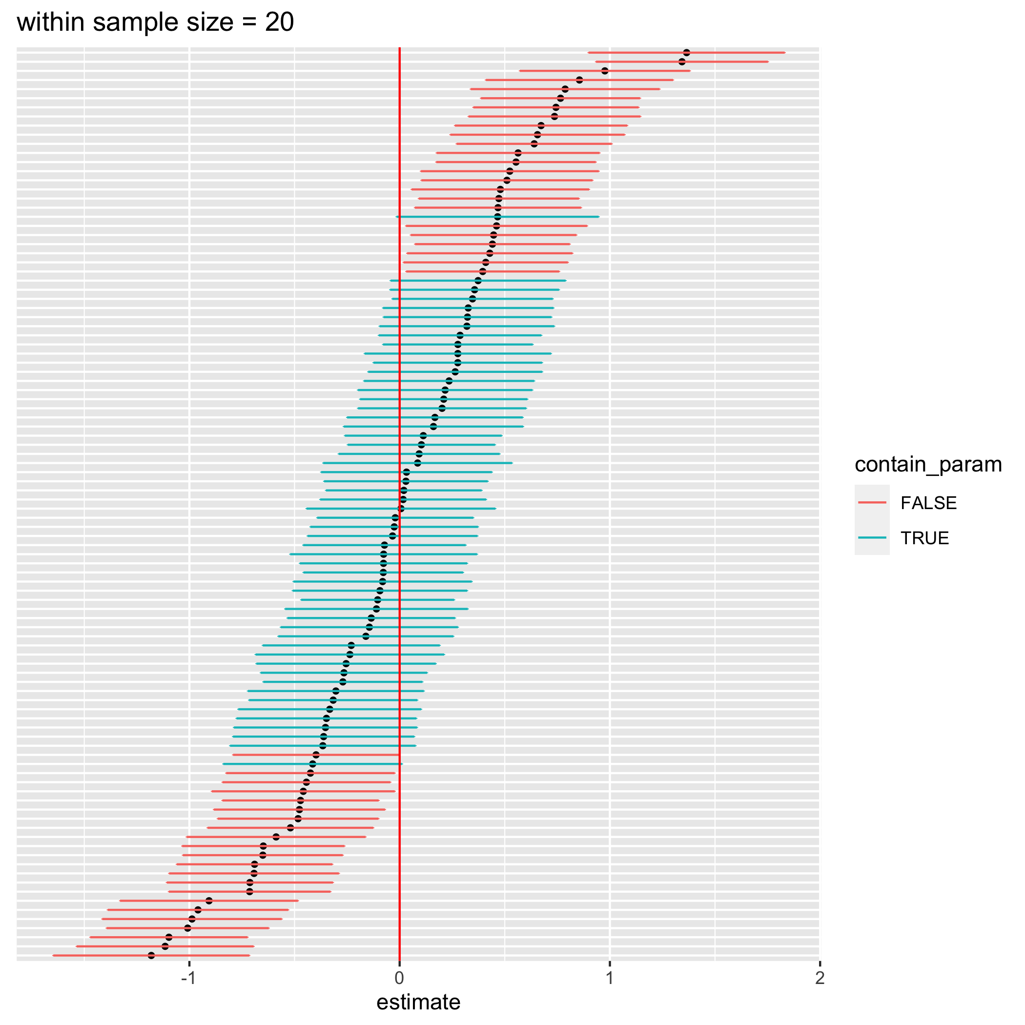
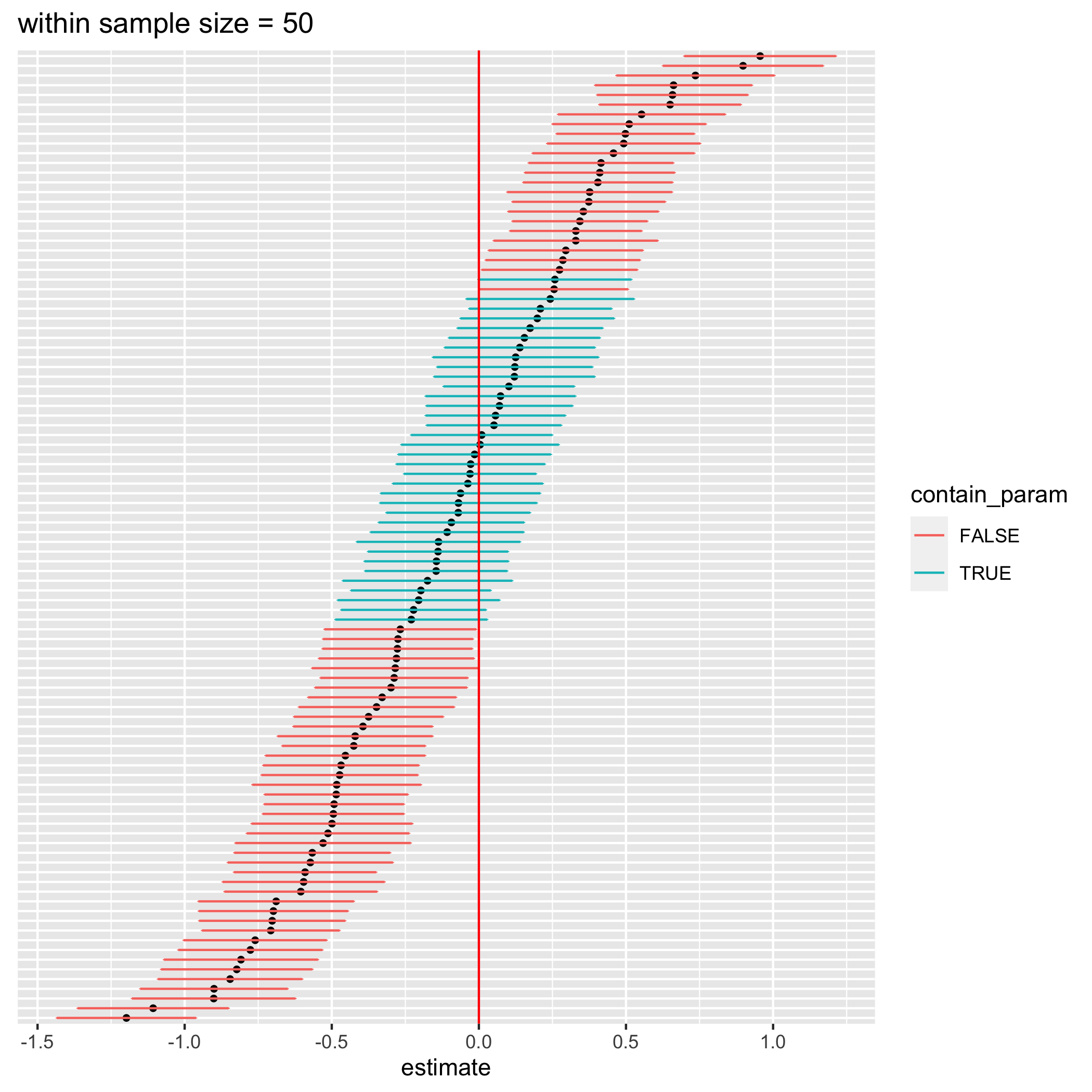
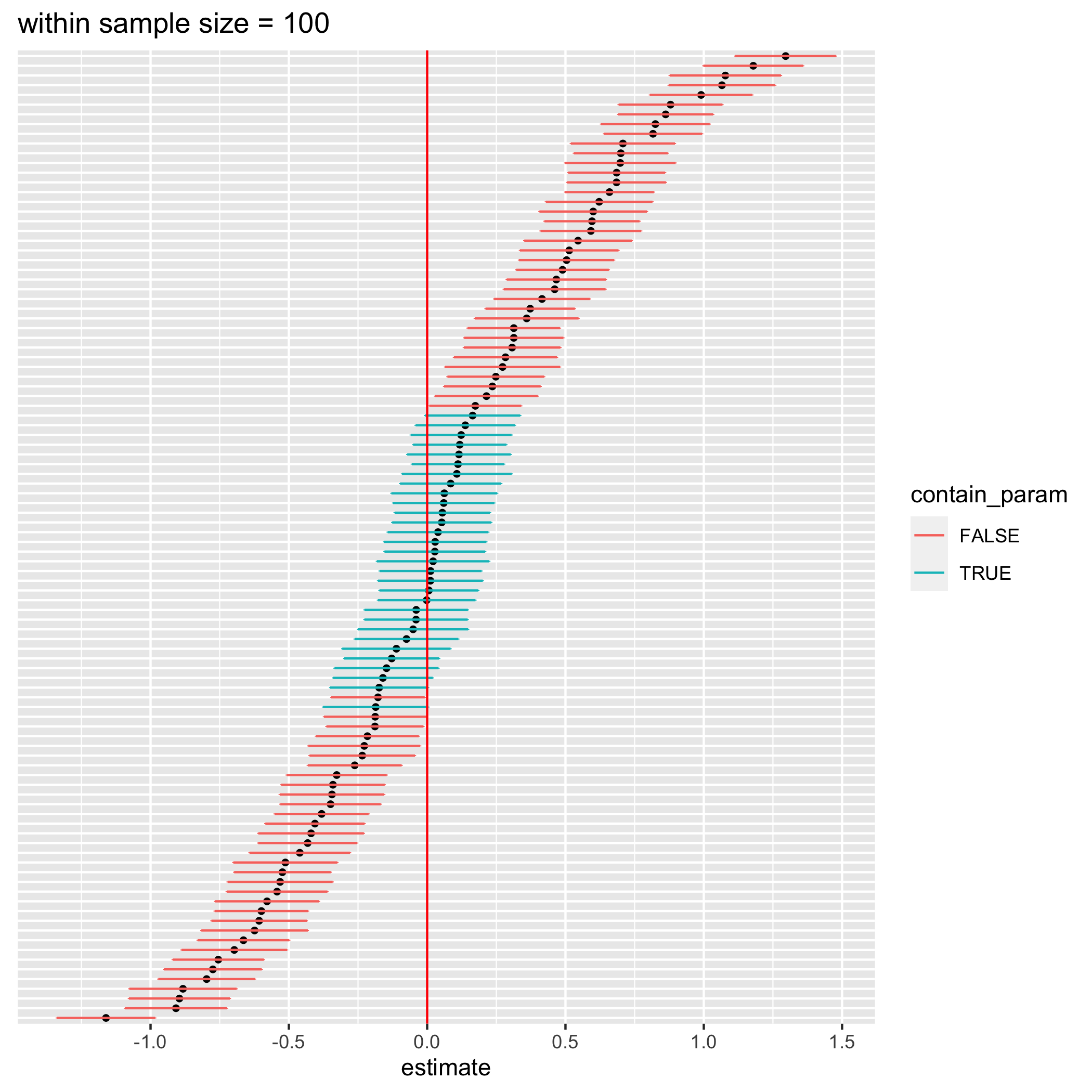
figure 1. 100 confidence intervals from simulated data with a) 20 data points per student, b) 50 data points per student, and c) 100 data points per student
I simulated data for the analysis 100 times and calculated their respective 95% confidence intervals for different number of data points per student (20, 50, and 100 from left to right figure). Each data point in each simulation represents an exam score of a student from a particular test. The results are shown in the figures above. According to the definition of confidence intervals, roughly 95 intervals should contain the true parameter, which is 0. However, most of the calculated confidence intervals don’t contain 0 at all (false statistical significance). Moreover, with more number of data points per student, there is less number of confidence intervals that actually contain 0. This happens because we ignore the variation in the effect of the tutoring class on different students resulting in more overconfidence intervals with larger sample sizes. Let’s try removing the variation of the between-student effect and redo the simulation again.
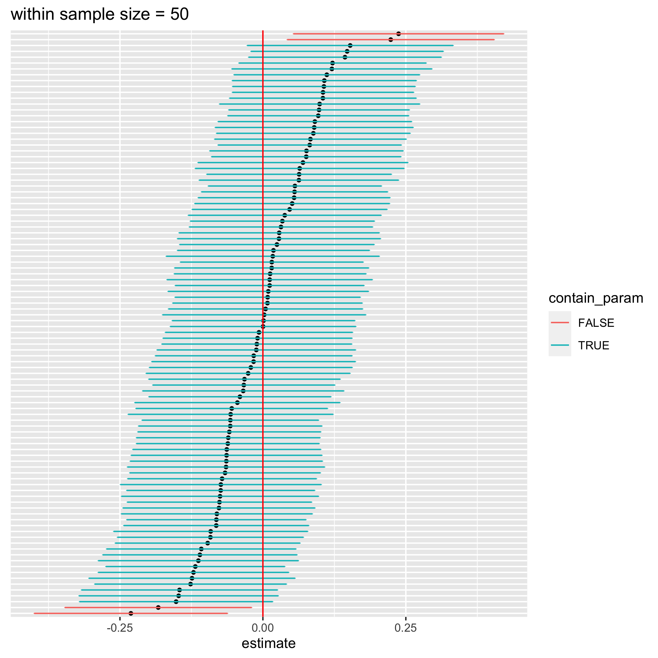
figure 2. 100 confidence intervals from a t-test of a non-varying effect between student data model
Now, most of the confidence intervals contain the true parameter value even with the t-test. But what if there’s a real variation in the between-student effect, and we want to account for it? A method to handle additional variance is to use multilevel/hierarchical/mixed effect model. This family of models will allow you to specify an additional level of data that causes a variation in the effect. In this example, that is the student-level variation. This model will also allow us to estimate effects for each level unit separately. Meaning, in this case, we can obtain the effect of the tutoring class for each individual student as well, but we will ignore them for now.
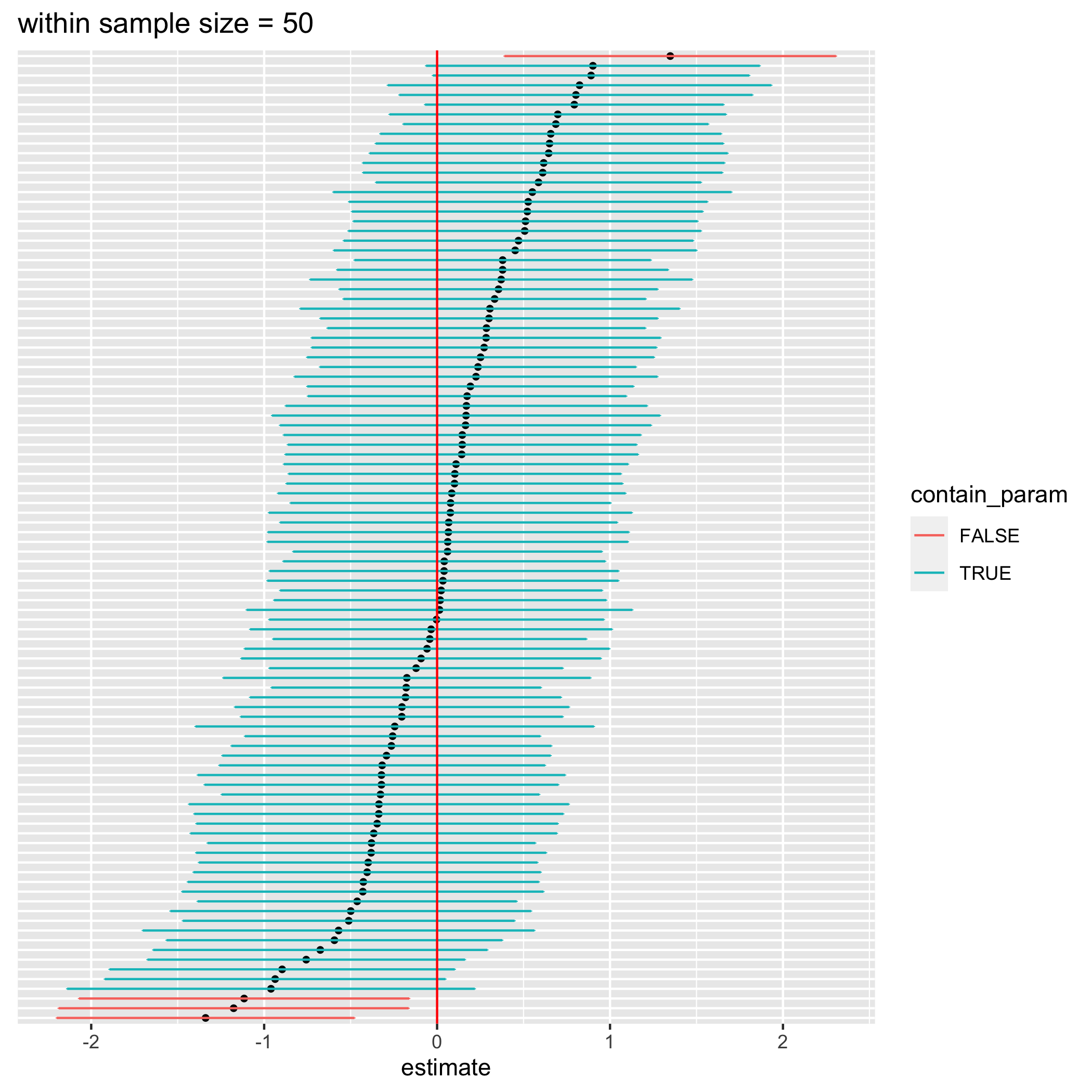
figure 3. 100 confidence intervals from an estimate in a mixed effect model when there’s a variation in tutoring effect between students
The above figure shows 95% confidence intervals of the tutoring effect when we use a mixed effect model instead of a t-test (or regular OLS). The confidence intervals become much wider (not overconfident) and contain the true parameter value (0) roughly 95% of the time now.
This is just one of many other scenarios that can throw off your confidence intervals and p-values. In reality, things are even more complicated than the example I used here. And anything can mess with your confidence intervals. I may write about them later when I feel motivated :)
One thing you should be aware of is that statistical inference with mixed effect model can be tricky and requires a specific algorithm to calculate confidence intervals and p-values. In the frequentist paradigm, once you move beyond traditional statistical tests, inferences (or the quantification of uncertainty) become more complicated, and there might not be ready-to-use tools to carry it out. Another thing is when you use the mixed effect model, the average effect could become a little less relevant. Do you care about the average effect or the individual-specific effect? The answer is can vary depending on your research question.
Extra notes
- This article is inspired by a preprint “generalizibility crisis” by Tal Yarkoni, in which he discusses issues that arise with mismatches between statistical models and verbal hypotheses more extensively https://doi.org/10.31234/osf.io/jqw35.
- Here’s the link to an R notebook that I used to produce analyses and figures for this article: https://htmlpreview.github.io/?https://raw.githubusercontent.com/chasnew/data_simulation_repo/master/unacc_var_mixedlm.html